Intermediate mathematics/Functions

Functions

A function f is like a "black box" that takes an input x, and returns a single corresponding output f(x).

The red curve is the graph of a function f in the Cartesian plane, consisting of all points with coordinates of the form (x, f(x)). The property of having one output for each input is represented geometrically by the fact that each vertical line (such as the yellow line through the origin) has exactly one crossing point with the curve.

From Wikipedia:Function (mathematics)

In mathematics, a function is a ^*relation between a ^*set of inputs and a set of permissible outputs with the property that each input is related to exactly one output. An example is the function $f(x)=x^2$ that relates each ^*real number x to its square x². The output of a function f corresponding to an input x is denoted by f(x) (read "f of x"). In this example, if the input is −3, then the output is 9, and we may write f(−3) = 9. See Tutorial:Evaluate by Substitution. Likewise, if the input is 3, then the output is also 9, and we may write f(3) = 9. (The same output may be produced by more than one input, but each input gives only one output.) The input ^*variable(s) are sometimes referred to as the argument(s) of the function.

Back to top

Euclids "common notions"

From Wikipedia:Euclidean geometry:

Things that do not differ from one another are equal to one another

a=a

Things that are equal to the same thing are also equal to one another

If

a=b b=c

then a=c

If equals are added to equals, then the wholes are equal

If

a=b c=d

then a+c=b+d

If equals are subtracted from equals, then the remainders are equal

If

a=b c=d

then a-c=b-d

The whole is greater than the part.

If

b≠0

then a+b>a

Back to top

Elementary algebra

ƒ(x) = x² is an example of an even function.

From Wikipedia:Elementary algebra:

Elementary algebra builds on and extends arithmetic by introducing letters called ^*variables to represent general (non-specified) numbers.

Algebraic expressions may be evaluated and simplified, based on the basic properties of arithmetic operations (addition^w, subtraction^w, multiplication^w, division^w and exponentiation^w). For example,

• Added terms are simplified using coefficients. For example, $x + x + x$ can be simplified as $3x$ (where 3 is a numerical coefficient).

• Multiplied terms are simplified using exponents. For example, $x \times x \times x$ is represented as $x^3$

• Like terms are added together, for example, $2x^2 + 3ab - x^2 + ab$ is written as $x^2 + 4ab$, because the terms containing $x^2$ are added together, and, the terms containing $ab$ are added together.

• Brackets can be "multiplied out", using the distributive property^w. For example, $x (2x + 3)$ can be written as $(x \times 2x) + (x \times 3)$ which can be written as $2x^2 + 3x$

• Expressions can be factored. For example, $6x^5 + 3x^2$, by dividing both terms by $3x^2$ can be written as $3x^2 (2x^3 + 1)$

ƒ(x) = x³ is an example of an odd function.

For any function $f$, if $a = b$ then:

• $f(a) = f(b)$
• $a + c = b + c$
• $ac = bc$
• $a^c = b^c$

One must be careful though when squaring both sides of an equation since this can result is solutions that dont satisfy the original equation.

$1 \neq -1$

yet

$1^2 = -1^2$

A function is an even function^w if f(x) = f(-x)

A function is an odd function^w if f(x) = -f(-x)

Back to top

Trigonometry

 

The law of cosines^w reduces to the Pythagorean theorem^w when gamma=90 degrees

$c^2 = a^2 + b^2 - 2ab\cos\gamma,$

The law of sines^w (also known as the "sine rule") for an arbitrary triangle states:

$\frac{a}{\sin A} = \frac{b}{\sin B} = \frac{c}{\sin C} = \frac{abc}{2\Delta},$

where $\Delta$ is the area of the triangle

$\mbox{Area} = \Delta = \frac{1}{2}a b\sin C.$

The law of tangents^w:

$\frac{a-b}{a+b}=\frac{\tan\left[\tfrac{1}{2}(A-B)\right]}{\tan\left[\tfrac{1}{2}(A+B)\right]}$

The parallelogram law reduces to the Pythagorean theorem when the parallelogram is a rectangle

$(AB)^2+(BC)^2+(CD)^2+(DA)^2=(AC)^2+(BD)^2\,$

Back to top

Right triangles

A right triangle is a triangle with gamma=90 degrees.

For small values of x, sin x ≈ x. (If x is in radians).

SOH → sin = "opposite" / "hypotenuse" CAH → cos = "adjacent" / "hypotenuse" TOA → tan = "opposite" / "adjacent"

= sin A = a/c = cos A = b/c = tan A = a/b

$\sin x = \frac{e^{ix} - e^{-ix}}{2i}, \qquad \cos x = \frac{e^{ix} + e^{-ix}}{2}, \qquad \tan x = \frac{i(e^{-ix} - e^{ix})}{e^{ix} + e^{-ix}}.$

(Note: the expression of tan(x) has i in the numerator, not in the denominator, because the order of the terms (and thus the sign) of the numerator is changed w.r.t. the expression of sin(x).)

Back to top

Hyperbolic functions

See also: ^*Hyperbolic angle

From Wikipedia:Hyperbolic function:

A ray through the ^*unit hyperbola $x^2 - y^2 = 1$ in the point $(\cosh a, \sinh a),$ where $a$ is twice the area between the ray, the hyperbola, and the $x$-axis. For points on the hyperbola below the $x$-axis, the area is considered negative (see animated version^w with comparison with the trigonometric (circular) functions).

Circle and hyperbola tangent at (1,1) display geometry of circular functions in terms of ^*circular sector area u and hyperbolic functions depending on ^*hyperbolic sector area u.

Hyperbolic functions^w are analogs of the ordinary trigonometric, or circular, functions.

• Hyperbolic sine:

$\sinh x = \frac {e^x - e^{-x}} {2} = \frac {e^{2x} - 1} {2e^x} = \frac {1 - e^{-2x}} {2e^{-x}}.$

• Hyperbolic cosine:

$\cosh x = \frac {e^x + e^{-x}} {2} = \frac {e^{2x} + 1} {2e^x} = \frac {1 + e^{-2x}} {2e^{-x}}.$

• Hyperbolic tangent:

$\tanh x = \frac{\sinh x}{\cosh x} = \frac {e^x - e^{-x}} {e^x + e^{-x}} =$

$= \frac{e^{2x} - 1} {e^{2x} + 1} = \frac{1 - e^{-2x}} {1 + e^{-2x}}.$

• Hyperbolic cotangent:

$\coth x = \frac{\cosh x}{\sinh x} = \frac {e^x + e^{-x}} {e^x - e^{-x}} =$

$= \frac{e^{2x} + 1} {e^{2x} - 1} = \frac{1 + e^{-2x}} {1 - e^{-2x}}, \qquad x \neq 0.$

• Hyperbolic secant:

$\operatorname{sech} x = \frac{1}{\cosh x} = \frac {2} {e^x + e^{-x}} =$

$= \frac{2e^x} {e^{2x} + 1} = \frac{2e^{-x}} {1 + e^{-2x}}.$

• Hyperbolic cosecant:

$\operatorname{csch} x = \frac{1}{\sinh x} = \frac {2} {e^x - e^{-x}} =$

$= \frac{2e^x} {e^{2x} - 1} = \frac{2e^{-x}} {1 - e^{-2x}}, \qquad x \neq 0.$

Back to top

Areas and volumes

The length of the circumference C of a circle is related to the radius r and diameter d by:

$\mathrm{Circumference} = \tau r = 2 \pi r = \pi d$

where

$\pi$ = 3.141592654

$\tau$ = 2 * π

The area of a circle is:

$\mathrm{Area} = \pi r^2$

The surface area of a sphere is

$\mathrm{\text{Surface area}} = 4 \cdot \pi r^2$

The surface area of a sphere 1 unit in radius is:

$4 \pi (1 \text{ unit})^2 = 12.56637 \text{ unit}^2$

The surface area of a sphere 128 units in radius is:

$4 \pi (128 \text{ unit})^2 = 205,887 \text{ unit}^2$

The volume inside a sphere is

$\mathrm{Volume} = \frac{4}{3} \cdot \pi r^3$

The volume of a sphere 1 unit in radius is:

$V = \frac{4}{3} \cdot \pi (1 \text{ unit})^3 = 4.1888 \text{ unit}^3$

The moment of inertia of a hollow sphere is:

$I = \frac{2}{3} m r^2\,\!$

Moment of inertia of a sphere is:

$I = \frac{2}{5} m r^2\,\!$

The area of a hexagon is:

$Area = \frac{3 \sqrt{3}}{2} a^2 = 2.59807621135 \cdot a^2$

where a is the length of any side.

Back to top

Fractals

A square that is twice as big is four times as massive because it is 2 dimensional (2² = 4). A cube that is twice as big is eight times as massive because it is 3 dimensional (2³ = 8).

A triangle that is twice as big is four times as massive.

But a Sierpiński triangle that is twice as big is exactly three times as massive. It therefore has a Hausdorff dimension of 1.5849. (2^1.5849 = 3)

A pyramid that is twice as big is eight times as massive.

But a Sierpiński pyramid that is twice as big is exactly five times as massive. It therefore has a Hausdorff dimension of 2.3219 (2^2.3219 = 5)

Back to top

Polynomials

See also: ^*Runge's phenomenon, ^*Polynomial ring, ^*System of polynomial equations, ^*Rational root theorem, ^*Descartes' rule of signs, and ^*Complex conjugate root theorem

From Wikipedia:Polynomial:

A polynomial^w can always be written in the form

$Z(x) = a_0 + a_1 x + a_2 x^2 + \dotsb + a_{n-1}x^{n-1} + a_n x^n$

where $a_0, \ldots, a_n$ are constants called coefficients and n is the degree^w of the polynomial.

A ^*linear polynomial is a polynomial of degree one.

Each individual ^*term is the product of the ^*coefficient and a variable raised to a nonnegative integer power.

A ^*monomial has only one term.

A ^*binomial has 2 terms.

^*Fundamental theorem of algebra:

Every single-variable, degree n polynomial with complex coefficients has exactly n complex roots^w.

However, some or even all of the roots might be the same number.

A root (or zero) of a function is a value of x for which Z(x)=0.

$Z(x) = a_n(x - z_1)(x - z_2)\dotsb(x - z_n)$

If $Z(x) = (x - z_1)(x - z_2)^k$ then z₂ is a root of ^*multiplicity k. z₂ is a root of multiplicity k-1 of the derivative (Derivative is defined below) of Z(x).

If k=1 then z₂ is a simple root.

The graph is tangent to the x axis at the multiple roots of f and not tangent at the simple roots.

The graph crosses the x-axis at roots of odd multiplicity and bounces off (not goes through) the x-axis at roots of even multiplicity.

Near x=z₂ the graph has the same general shape as $A(x - z_2)^k$

The ^*complex conjugate root theorem states that if the coefficients of a polynomial are real, then the non-real roots appear in pairs of the form (a + ib, a – ib).

The roots of the formula $ax^{2} + bx + c = 0$ are given by the Quadratic formula^w:

$x = \frac{-b \pm \sqrt{b^2 - 4ac}}{2a}.$ See Completing the squarew

$b^2 - 4ac$ is called the discriminant.

$ax^2+bx+c \quad = \quad a(x+\frac{b}{2a})^2+c-\frac{b^2}{4a} \quad = \quad a(x-h)^2+k$

This is a parabola shifted to the right h units, stretched by a factor of a, and moved upward k units.

k is the value at x=h and is either the maximum or the minimum value.

The roots of

$a_0 + a_1 x + \cdots + a_n x^n,$

are the multiplicative inverses of

$a_n + a_{n-1} x + \cdots + a_0 x^n,$

There is no formula for the roots of a fifth (or higher) degree polynomial equation in terms of the coefficients of the polynomial, using only the usual algebraic operations (addition, subtraction, multiplication, division) and application of radicals (square roots, cube roots, etc). See ^*Galois theory.

^*Binomial therorem:

$(x+y)^n = {n \choose 0}x^n y^0 + {n \choose 1}x^{n-1}y^1 + {n \choose 2}x^{n-2}y^2 + \cdots + {n \choose n-1}x^1 y^{n-1} + {n \choose n}x^0 y^n,$

Where $\binom{n}{k} = \frac{n!}{k! (n-k)!}.$ See Binomial coefficient^w

Isaac Newton generalized the binomial theorem to allow real exponents other than nonnegative integers. (The same generalization also applies to complex exponents.) In this generalization, the finite sum is replaced by an infinite series.

$x^2 - y^2 = (x + y)(x - y)$

$x^2 + y^2 = (x + yi)(x - yi)$

The polynomial remainder theorem^w states that the remainder of the division of a polynomial Z(x) by the linear polynomial x-a is equal to Z(a). See ^*Ruffini's rule.

Determining the value at Z(a) is sometimes easier if we use ^*Horner's method (^*synthetic division) by writing the polynomial in the form

$Z(x) = a_0 + x(a_1 + x(a_2 + \cdots + x(a_{n-1} + x(a_n)))).$

A ^*monic polynomial is a one variable polynomial in which the leading coefficient is equal to 1.

$a_0 + a_1x + a_2x^2 + \cdots + a_{n-1}x^{n-1} + 1x^n$

Back to top

Rational functions

A ^*rational function is a function of the form

$f(x) = k{(x - z_1)(x - z_2)\dotsb(x - z_n) \over (x - p_1)(x - p_2)\dotsb(x - p_m)} = {Z(x) \over P(x)}$

It has n zeros^w and m poles^w. A pole is a value of x for which |f(x)| = infinity.

The vertical asymptotes^w are the poles of the rational function.

If n<m then f(x) has a horizontal asymptote at the x axis

If n=m then f(x) has a horizontal asymptote at k.

If n>m then f(x) has no horizontal asymptote.

See also ^*Wikipedia:Asymptote#Oblique_asymptotes

Given two polynomials $Z(x)$ and $P(x) = (x-p_1)(x-p_2) \cdots (x-p_m)$, where the p_i are distinct constants and deg Z < m, partial fractions^w are generally obtained by supposing that

$\frac{Z(x)}{P(x)} = \frac{c_1}{x-p_1} + \frac{c_2}{x-p_2} + \cdots + \frac{c_m}{x-p_m}$

and solving for the c_i constants, by substitution, by ^*equating the coefficients of terms involving the powers of x, or otherwise.

(This is a variant of the ^*method of undetermined coefficients.)

If the degree of Z is not less than m then use long division to divide P into Z. The remainder then replaces Z in the equation above and one proceeds as before.

If $P(x) = (x-p)^m$ then $\frac{Z(x)}{P(x)} = \frac{c_1}{(x-p)} + \frac{c_2}{(x-p)^2} + \cdots + \frac{c_m}{(x-p)^m}$

A ^*Generalized hypergeometric series is given by

$\sum_{x=0} c_x$ where c₀=1 and ${c_{x+1} \over c_x} = {Z(x) \over P(x)} = f(x)$

The function f(x) has n zeros and m poles.

^*Basic hypergeometric series, or hypergeometric q-series, are ^*q-analogue generalizations of generalized hypergeometric series.

Roughly speaking a ^*q-analog of a theorem, identity or expression is a generalization involving a new parameter q that returns the original theorem, identity or expression in the limit as q → 1

We define the q-analog of n, also known as the q-bracket or q-number of n, to be

$[n]_q=\frac{1-q^n}{1-q} = q^0 + q^1 + q^2 + \ldots + q^{n - 1}$

one may define the q-analog of the factorial^w, known as the ^*q-factorial, by

$[n]_q! = [1]_q \cdot [2]_q \cdots [n-1]_q \cdot [n]_q$

^*Elliptic hypergeometric series are generalizations of basic hypergeometric series.

An elliptic function is a meromorphic function that is periodic in two directions.

A ^*generalized hypergeometric function is given by

$F(x) = {}_nF_m(z_1,...z_n;p_1,...p_m;x) = \sum_{y=0} c_y x^y$

So for e^x (see below) we have:

$c_y = \frac{1}{y!}, \qquad \frac{c_{y+1}}{c_y} = \frac{1}{y+1}.$

Back to top

Integration and differentiation

Force • distance = energy

See also: Hyperreal number^w and Implicit differentiation^w

The integral^w is a generalization of multiplication.

For example: a unit mass dropped from point x₂ to point x₁ will release energy.

The usual equation is is a simple multiplication:

$gravity \cdot (x_2 - x_1) = energy$

But that equation cant be used if the strength of gravity is itself a function of x.

The strength of gravity at x₁ would be different than it is at x₂.

And in reality gravity really does depend on x (x is the distance from the center of the earth):

$gravity(x) = 1/x^2$ (See inverse-square law^w.)

However, the corresponding Definite integral^w is easily solved:

$\int_{x_1}^{x_2} gravity(x) \cdot dx$

The surprisingly simple rules for solving definite integrals

$\int_{x_1}^{x_2} f(x) \cdot dx \quad = \quad F(x_2)-F(x_1)$ F(x) is called the indefinite integralw. (antiderivativew) $F(x) = \int f(x) \cdot dx$ k and y are arbitrary constants: $\int k \cdot x^y \cdot dx \quad = \quad k \cdot \int x^y \cdot dx \quad = \quad k \cdot \frac{x^{y+1}}{y+1}$ (Units (feet, mm...) behave exactly like constants.) And most conveniently : $\int \bigg (f(x) + g(x) \bigg) \cdot dx = \int f(x) \cdot dx + \int g(x) \cdot dx$

The integral of a function is equal to the area under the curve.

When the "curve" is a constant (in other words, k•x⁰) then the integral reduces to ordinary multiplication.

The derivative^w is a generalization of division.

The derivative of the integral of f(x) is just f(x).

The derivative of a function at any point is equal to the slope of the function at that point.

$f'(x)=\frac{f(x+dx)-f(x)}{dx}.$

The equation of the line tangent to a function at point a is

$y(x) = f(a) + f'(a)(x-a)$

The Lipschitz constant^w of a function is a real number for which the absolute value of the slope of the function at every point is not greater than this real number.

The derivative of f(x) where f(x) = k•x^y is

$f'(x) = {df \over dx} = {d(k \cdot x^y) \over dx} \quad = \quad k \cdot {d(x^y) \over dx} \quad = \quad k \cdot y \cdot x^{y-1}$

The derivative of a $k \cdot x^0$ is $k \cdot 0 \cdot x^{-1}$

The integral of $x^{-1}$ is ln(x). See natural log^w

Chain rule^w for the derivative of a function of a function:

$f(g(x))' = \frac{df}{dx} = \frac{df}{dg} \cdot \frac{dg}{dx}$

The Chain rule for a function of 2 functions:

$f(g(x), h(x))' = \frac{\operatorname df}{\operatorname dx} = { \partial f \over \partial g}{\operatorname dg \over \operatorname dx} + {\partial f \over \partial h}{\operatorname dh \over \operatorname dx }$ (See "partial derivatives" below)

The Product rule^w can be considered a special case of the chain rule^w for several variables

$\frac{df}{dx} = {d (g(x) \cdot h(x)) \over dx} = \frac{\partial(g \cdot h)}{\partial g}\frac{dg}{dx}+\frac{\partial (g \cdot h)}{\partial h}\frac{dh}{dx} = \frac{dg}{dx} h + g \frac{dh}{dx}$

Product rule^w:

$(g \cdot h)' = \frac{(g+dg) \cdot (h+dh) - g \cdot h}{dx} = g' \cdot h + g \cdot h'$ (because $dh \cdot dg$ is negligible)

$(g \cdot h \cdot j)' = g' \cdot h \cdot j + g \cdot h' \cdot j + g \cdot h \cdot j'$

^*General Leibniz rule:

$(gh)^{(n)}=\sum_{k=0}^n {n \choose k} g^{(n-k)} h^{(k)}$

By the chain rule:

$\bigg(\frac{1}{h}\bigg)' = \frac{-1}{h^2} \cdot h'$

Therefore the Quotient rule^w:

$\bigg( \frac{g(x)}{h(x)} \bigg)' = \bigg( g \cdot \frac{1}{h} \bigg)' = g' \cdot \frac{1}{h} + g \cdot \frac{-h'}{h^2} = \frac{g' \cdot h - g \cdot h'}{h^2}$

There is a chain rule for integration but the inner function must have the form $g=ax+c$ so that its derivative $\frac{dg}{dx} = a$ and therefore $dx=\frac{dg}{a}$

$\int f(g(x)) \cdot dx = \int f(g) \cdot \frac{dg}{a} = \frac{1}{a} \int f(g) \cdot dg$

Actually the inner function can have the form $g=ax^y+c$ so that its derivative $\frac{dg}{dx} = a \cdot y \cdot x^{y-1}$ and therefore $dx=\frac{dg}{a \cdot y \cdot x^{y-1}}$ provided that all factors involving x cancel out.

$\int x^{y-1} \cdot f(g(x)) \cdot dx = \int {\color{red} x^{y-1}} \cdot f(g) \cdot \frac{dg}{a \cdot y \cdot {\color{red} x^{y-1}}} = \frac{1}{a \cdot y} \int f(g) \cdot dg$

The product rule for integration is called Integration by parts^w

$g \cdot h' = (g \cdot h)' - g' \cdot h$

$\int g \cdot h' \cdot dx = g \cdot h - \int g' \cdot h \cdot dx$

One can use partial fractions^w or even the Taylor series^w to convert difficult integrals into a more manageable form.

$\frac{f(x)}{(x-1)^2} = \frac{a_0(x-1)^0 + a_1(x-1)^1 + \dots + a_n(x-1)^n}{(x-1)^2}$

The fundamental theorem of Calculus is:

$F(x) - F(a) = \int_a^x\!f(t)\, dt \quad \text{and} \quad F'(x) = f(x)$

The fundamental theorem of calculus is just the particular case of the ^*Leibniz integral rule:

$\frac{d}{dx} \left (\int_{a(x)}^{b(x)}f(x,t)\,dt \right) = f\big(x,b(x)\big)\cdot \frac{d}{dx} b(x) - f\big(x,a(x)\big)\cdot \frac{d}{dx} a(x) + \int_{a(x)}^{b(x)}\frac{\partial}{\partial x} f(x,t) \,dt.$

In calculus, a function f defined on a subset of the real numbers with real values is called ^*monotonic if and only if it is either entirely non-increasing, or entirely non-decreasing.

A differential form^w is a generalisation of the notion of a differential^w that is independent of the choice of ^*coordinate system. f(x,y) dx ∧ dy is a 2-form in 2 dimensions (an area element). The derivative^w operation on an n-form is an n+1-form; this operation is known as the exterior derivative^w. By the generalized Stokes' theorem^w, the integral of a function over the boundary of a manifold^w is equal to the integral of its exterior derivative on the manifold itself.

Back to top

Taylor & Maclaurin series

If we know the value of a smooth function^w at x=0 (smooth means all its derivatives are continuous^w) and we also know the value of all of its derivatives at x=0 then we can determine the value at any other point x by using the Maclaurin series^w. ("!" means factorial^w)

$f(x) = a_0 x^0 + a_1 x^1 + a_2 x^2 + a_3 x^3 \cdots \quad \text{where} \quad a_n = {f^{(n)}(0) \over n!}$

The proof of this is actually quite simple. Plugging in a value of x=0 causes all terms but the first to become zero. So, assuming that such a function exists, a₀ must be the value of the function at x=0. Simply differentiate both sides of the equation and repeat for the next term. And so on.

Because the functions $x^n$ can be multiplied by scalars and added they therefore form an infinite dimensional vector space. (An infinite dimensional space is not a ^*Compact space.) The function f(x) occupies a single point in that infinite dimensional space corresponding to a vector whose components are $a_n$

$\mathbf{v} = \begin{bmatrix} a_0 & a_1 & a_2 & \ldots & a_{\infty} \end{bmatrix}$

The Taylor series^w generalizes the Maclaurin series.

$f(z)=\sum_{k=0}^\infty \alpha_k (z-z_0)^k$

Riemann surface for the function ƒ(z) = √z. For the imaginary part rotate 180°.

An analytic function^w is a function whose Taylor series converges for every z₀ in its domain^w; analytic functions are infinitely differentiable^w.

Any vector g = (z₀, α₀, α₁, ...) is a ^*germ if it represents a power series of an analytic function^w around z₀ with some radius of convergence r > 0.

The set of germs $\mathcal G$ is a Riemann surface^w.

Riemann surfaces are the objects on which multi-valued functions become single-valued.

A ^*connected component of $\mathcal G$ (i.e., an equivalence class) is called a ^*sheaf.

We can easily determine the Maclaurin series expansion of the exponential function^w $e^x$ because it is equal to its own derivative.

$e^x = \sum_{n = 0}^{\infty} {x^n \over n!} = {x^0 \over 0!} + {x^1 \over 1!} + {x^2 \over 2!} + {x^3 \over 3!} + {x^4 \over 4!} + \cdots$

The above holds true even if x is a matrix. See ^*Matrix exponential

And likewise for cos(x)^w and sin(x)^w because cosine is the derivative of sine which is the derivative of -cosine

$\cos x = \frac{x^0}{0!} - \frac{x^2}{2!} + \frac{x^4}{4!} - \frac{x^6}{6!} + \cdots$

$\sin x = \frac{x^1}{1!} - \frac{x^3}{3!} + \frac{x^5}{5!} - \frac{x^7}{7!} + \cdots$

It then follows that $e^{ix}=\cos x+i\sin x=\operatorname{cis} x$ and therefore $e^{i \pi}=-1 + i\cdot0$ See Euler's formula^w

x is the angle in ^*radians.

This makes the equation for a circle in the complex plane, and by extension sine and cosine, extremely simple and easy to work with especially with regard to differentiation and integration.

$\frac{d(e^{i \cdot k \cdot t})}{dt} = i \cdot k \cdot e^{i \cdot k \cdot t}$

For sine waves differentiation and integration are replaced with multiplication and division. Calculus is replaced with algebra. Therefore any expression that can be represented as a sum of sine waves can be easily differentiated or integrated.

Back to top

Fourier Series

The Maclaurin series cant be used for a discontinuous function like a square wave because it is not differentiable. (^*Distributions make it possible to differentiate functions whose derivatives do not exist in the classical sense. See ^*Generalized function.)

But remarkably we can use the Fourier series^w to expand it or any other periodic function^w into an infinite sum of sine waves each of which is fully differentiable^w!

$f(t) = \frac{a_0}{2} + \sum_{n=1}^\infty \left[a_n\cos\left(nt\right)+b_n\sin\left(nt\right)\right]$

$a_n = \frac{2}{p}\int_{t_0}^{t_p} f(t)\cdot \cos\left(\tfrac{2\pi nt}{p}\right)\ dt$

$b_n = \frac{2}{p}\int_{t_0}^{t_p} f(t)\cdot \sin\left(\tfrac{2\pi nt}{p}\right)\ dt$

A square wave consists of all odd frequencies with the amplitude of each frequency being $\frac{1}{f}$.

A dirac comb consists of all integer frequencies with the amplitude of each frequency being 1.

sin²(x) = 0.5*cos(0x) - 0.5*cos(2x)

The reason this works is because sine and cosine are ^*orthogonal functions.

Two vectors are said to be orthogonal when:

$\mathbf{u} \cdot \mathbf{v} = 0$

or more generally when:

$\beta(\mathbf{u,v}) = 0$

Two functions are said to be orthogonal when:

$\langle f,g \rangle = \int \overline{f(x)}g(x)\,dx = 0.$

That means that multiplying any 2 sine waves of frequency n and frequency m and integrating over one period will always equal zero unless n=m.

See the graph of sin²(x) to the right.

$\sin mx \cdot \sin nx = \frac{\cos (m - n)x - \cos (m+n) x}{2}$

See ^*Amplitude_modulation

And of course ∫ f_n*(f₁+f₂+f₃+...) = ∫ (f_n*f₁) + ∫ (f_n*f₂) + ∫ (f_n*f₃) +...

The complex form of the Fourier series uses complex exponentials instead of sine and cosine and uses both positive and negative frequencies (clockwise and counter clockwise) whose imaginary parts cancel.

The complex coefficients encode both amplitude and phase and are complex conjugates of each other.

$F(\nu) = \mathcal{F}\{f\} = \int_{\mathbb{R}^n} f(x) e^{-2 \pi i x\cdot\nu} \, \mathrm{d}x$

where the dot between x and ν indicates the inner product^w of Rⁿ.

A 2 dimensional Fourier series is used in video compression.

A ^*discrete Fourier transform can be computed very efficiently by a ^*fast Fourier transform (FFT).

The FFT has been described as "the most important numerical algorithm of our lifetime"

In mathematical analysis, many generalizations of Fourier series have proven to be useful.

They are all special cases of decompositions over an orthonormal basis of an inner product space.

^*Spherical harmonics are a complete set of orthogonal functions on the sphere, and thus may be used to represent functions defined on the surface of a sphere, just as circular functions (sines and cosines) are used to represent functions on a circle via Fourier series.

Spherical harmonics are ^*basis functions for SO(3). See Laplace series^w.

Every continuous function in the function space can be represented as a ^*linear combination of basis functions, just as every vector in a vector space can be represented as a linear combination of basis vectors.

Every quadratic polynomial can be written as a1+bt+ct², that is, as a linear combination of the basis functions 1, t, and t².

Back to top

Transforms

Fourier transforms^w generalize Fourier series to nonperiodic functions like a single pulse of a square wave.

The more localized in the time domain (the shorter the pulse) the more the Fourier transform is spread out across the frequency domain and vice versa, a phenomenon known as the uncertainty principle^w.

Using the Fourier transform we can determine that the Dirac delta function^w consists of all frequencies with the amplitude of each frequency being 1.

$G(\omega)=\mathcal{F}\{f(t)\}=\int_{-\infty}^\infty f(t) e^{-i\omega t}dt$

Laplace transforms^w generalize Fourier transforms to complex frequency $s=\sigma+i\omega$.

Complex frequency includes a term corresponding to the amount of damping.

See http://www.dspguide.com/CH32.PDF.

$F(s)=\mathcal{L}\{f(t)\}=\int_0^\infty f(t) e^{-\sigma t}e^{-i \omega t}dt$

$\mathcal{L}\{ \delta(t-a) \} = e^{-as}$, (assuming a > 0)

$\mathcal{L}\{e^{at} \}= \frac{1}{s - a}$

The inverse Laplace transform^w is given by

$f(t) = \mathcal{L}^{-1} \{F\} = \frac{1}{2\pi i}\lim_{T\to\infty}\int_{\gamma-iT}^{\gamma+iT}F(s)e^{st}\,ds,$

where the integration is done along the vertical line Re(s) = γ in the complex plane^w such that γ is greater than the real part of all ^*singularities of F(s) and F(s) is bounded on the line, for example if contour path is in the ^*region of convergence.

If all singularities are in the left half-plane, or F(s) is an ^*entire function , then γ can be set to zero and the above inverse integral formula becomes identical to the ^*inverse Fourier transform.

The ^*Z-transform can be considered as a discrete-time equivalent of the Laplace transform. This similarity is explored in the theory of ^*time-scale calculus.

Integral transforms^w generalize Fourier transforms to other ^*kernals (besides sine^w and cosine^w)

Cauchy kernel =$\frac{1}{\zeta-x} \quad \text{or} \quad \frac{1}{2\pi i} \cdot \frac{1}{\zeta-x}$

Hilbert kernel = $cot\frac{\theta-t}{2}$

Poisson Kernel:

For the ball of radius r, $B_{r}$, in Rⁿ, the Poisson kernel takes the form:

$P(x,\zeta) = \frac{r^2-|x|^2}{r} \cdot \frac{1}{|\zeta-x|^n} \cdot \frac{1}{\omega_{n}}$

where $x\in B_{r}$, $\zeta\in S$ (the surface of $B_{r}$), and $\omega_n$ is the ^*surface area of the unit n-sphere.

unit disk (r=1) in the complex plane:

$K(x,\phi) = \frac{1^2-|x|^2}{1} \cdot \frac{1}{|e^{i\phi}-x|^2}\cdot \frac{1}{2\pi}$

Dirichlet kernel

$D_n(x)=\sum_{k=-n}^n e^{ikx}=1+2\sum_{k=1}^n\cos(kx)=\frac{\sin\left(\left(n + \frac{1}{2}\right) x \right)}{\sin(\frac{x}{2})} \approx 2\pi\delta(x)$

The ^*convolution theorem states that

$\mathcal{F}\{f*g\} = \mathcal{F}\{f\} \cdot \mathcal{F}\{g\}$

where $\cdot$ denotes point-wise multiplication. It also works the other way around:

$\mathcal{F}\{f \cdot g\}= \mathcal{F}\{f\}*\mathcal{F}\{g\}$

By applying the inverse Fourier transform $\mathcal{F}^{-1}$, we can write:

$f*g= \mathcal{F}^{-1}\big\{\mathcal{F}\{f\}\cdot\mathcal{F}\{g\}\big\}$

and:

$f \cdot g= \mathcal{F}^{-1}\big\{\mathcal{F}\{f\}*\mathcal{F}\{g\}\big\}$

This theorem also holds for the Laplace transform^w.

The ^*Hilbert transform is a ^*multiplier operator. The multiplier of H is σ_H(ω) = −i sgn(ω) where sgn is the ^*signum function. Therefore:

$\mathcal{F}(H(u))(\omega) = (-i\,\operatorname{sgn}(\omega)) \cdot \mathcal{F}(u)(\omega)$

where $\mathcal{F}$ denotes the Fourier transform^w.

Since sgn(x) = sgn(2πx), it follows that this result applies to the three common definitions of $\mathcal{F}$.

By Euler's formula^w,

$\sigma_H(\omega) = \begin{cases} i = e^{+\frac{i\pi}{2}}, & \text{for } \omega < 0\\ 0, & \text{for } \omega = 0\\ -i = e^{-\frac{i\pi}{2}}, & \text{for } \omega > 0 \end{cases}$

Therefore, H(u)(t) has the effect of shifting the phase of the ^*negative frequency components of u(t) by +90° (π/2 radians) and the phase of the positive frequency components by −90°.

And i·H(u)(t) has the effect of restoring the positive frequency components while shifting the negative frequency ones an additional +90°, resulting in their negation.

In electrical engineering, the convolution of one function (the input signal) with a second function (the impulse response) gives the output of a linear time-invariant system (LTI).

At any given moment, the output is an accumulated effect of all the prior values of the input function

Back to top

Differential equations

See also: ^*Variation of parameters

Simple harmonic motion shown both in real space and ^*phase space.

^*Simple harmonic motion of a mass on a spring is a second-order linear ordinary differential equation^w.

$Force = mass*acc = m\frac{\mathrm{d}^2 x}{\mathrm{d}t^2} = -kx,$

where m is the inertial mass, x is its displacement from the equilibrium, and k is the spring constant.

Solving for x produces

$x(t) = A\cos\left(\omega t - \varphi\right),$

A is the amplitude (maximum displacement from the equilibrium position), $\omega = 2\pi f = \sqrt{k/m}$ is the angular frequency^w, and φ is the phase.

Energy passes back and forth between the potential energy in the spring and the kinetic energy of the mass.

The important thing to note here is that the frequency of the oscillation depends only on the mass and the stiffness of the spring and is totally independent of the amplitude.

That is the defining characteristic of resonance.

RLC series circuit

^*Kirchhoff's voltage law states that the sum of the emfs in any closed loop of any electronic circuit is equal to the sum of the ^*voltage drops in that loop.

$V(t) = V_R + V_L + V_C$

V is the voltage, R is the resistance, L is the inductance, C is the capacitance.

$V(t) = RI(t) + L \frac{dI(t)}{dt} + \frac{1}{C} \int_{0}^t I(\tau)\, d\tau$

I = dQ/dt is the current.

It makes no difference whether the current is a small number of charges moving very fast or a large number of charges moving slowly.

In reality ^*the latter is the case.

^*Damping oscillation is a typical ^*transient response

If V(t)=0 then the only solution to the equation is the transient response which is a rapidly decaying sine wave with the same frequency as the resonant frequency of the circuit.

Like a mass (inductance) on a spring (capacitance) the circuit will resonate at one frequency.

Energy passes back and forth between the capacitor and the inductor with some loss as it passes through the resistor.

If V(t)=sin(t) from -∞ to +∞ then the only solution is a sine wave with the same frequency as V(t) but with a different amplitude and phase.

If V(t) is zero until t=0 and then equals sin(t) then I(t) will be zero until t=0 after which it will consist of the steady state response plus a transient response.

From Wikipedia:Characteristic equation (calculus):

Starting with a linear homogeneous differential equation with constant coefficients $a_{n}, a_{n-1}, \ldots , a_{1}, a_{0}$,

$a_{n}y^{(n)} + a_{n-1}y^{(n-1)} + \cdots + a_{1}y^\prime + a_{0}y = 0$

it can be seen that if $y(x) = e^{rx} \,$, each term would be a constant multiple of $e^{rx} \,$. This results from the fact that the derivative of the exponential function^w $e^{rx} \,$ is a multiple of itself. Therefore, $y' = re^{rx} \,$, $y'' = r^{2}e^{rx} \,$, and $y^{(n)} = r^{n}e^{rx} \,$ are all multiples. This suggests that certain values of $r \,$ will allow multiples of $e^{rx} \,$ to sum to zero, thus solving the homogeneous differential equation. In order to solve for $r \,$, one can substitute $y = e^{rx} \,$ and its derivatives into the differential equation to get

$a_{n}r^{n}e^{rx} + a_{n-1}r^{n-1}e^{rx} + \cdots + a_{1}re^{rx} + a_{0}e^{rx} = 0$

Since $e^{rx} \,$ can never equate to zero, it can be divided out, giving the characteristic equation

$a_{n}r^{n} + a_{n-1}r^{n-1} + \cdots + a_{1}r + a_{0} = 0$

By solving for the roots, $r \,$, in this characteristic equation, one can find the general solution to the differential equation. For example, if $r \,$ is found to equal to 3, then the general solution will be $y(x) = ce^{3x} \,$, where $c \,$ is an arbitrary constant^w.

Back to top

Partial derivatives

See also: ^*Currying

^*Partial derivatives and ^*multiple integrals generalize derivatives and integrals to multiple dimensions.

The partial derivative with respect to one variable $\frac{\part f(x,y)}{\part x}$ is found by simply treating all other variables as though they were constants.

Multiple integrals are found the same way.

Let f(x, y, z) be a scalar function^w (for example electric potential energy or temperature).

A 2 dimensional example of a scalar function would be an elevation map.

(Contour lines of an elevation map are an example of a ^*level set.)

The total derivative^w of f(x(t), y(t)) with respect to t is

$\frac{\operatorname df}{\operatorname dt} = { \partial f \over \partial x}{\operatorname dx \over \operatorname dt} + {\partial f \over \partial y}{\operatorname dy \over \operatorname dt }$

And the differential^w is

$\operatorname df = { \partial f \over \partial x}\operatorname dx + {\partial f \over \partial y} \operatorname dy .$

Back to top

Gradient of scalar field

The Gradient^w of f(x, y, z) is a vector field whose value at each point is a vector (technically its a covector^w because it has units of distance⁻¹) that points "downhill" with a magnitude equal to the slope^w of the function at that point.

You can think of it as how much the function changes per unit distance.

The gradient of temperature gives heat flow.

$\operatorname{grad}(f) = \nabla f = \frac{\partial f}{\partial x} \mathbf{i} + \frac{\partial f}{\partial y} \mathbf{j} + \frac{\partial f}{\partial z} \mathbf{k} = \mathbf{F}$

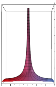
For static (unchanging) fields the Gradient of the electric potential is the electric field^w itself. Image below shows the potential of a single point charge.

Its gradient gives the electric field which is shown in the 2 images below. In the image on the left the field strength is proportional to the length of the vectors. In the image on the right the field strength is proportional to the density of the ^*flux lines. The image is 2 dimensional and therefore the flux density in the image follows an inverse first power law but in reality the field lines from a real proton or electron spread outward in 3 dimensions and therefore follow an inverse square law. Inverse square means that at twice the distance the field is four times weaker.

The field of 2 point charges is simply the linear sum of the separate charges.

Back to top

Divergence

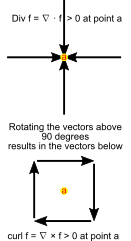
The Divergence^w of a vector field is a scalar.

The divergence of the electric field is non-zero wherever there is electric charge^w and zero everywhere else.

^*Field lines begin and end at charges because the charges create the electric field.

$\operatorname{div}\,\mathbf{F} = {\color{red} \nabla\cdot\mathbf{F} } = \left( \frac{\partial}{\partial x}, \frac{\partial}{\partial y}, \frac{\partial}{\partial z} \right) \cdot (F_x,F_y,F_z) = \frac{\partial F_x}{\partial x} +\frac{\partial F_y}{\partial y} +\frac{\partial F_z}{\partial z}.$

The Laplacian^w is the divergence of the gradient of a function:

$\Delta f = \nabla^2 f = (\nabla \cdot \nabla) f = \frac{\partial^2 f}{\partial x^2} + \frac{\partial^2 f}{\partial y^2} + \frac{\partial^2 f}{\partial z^2}.$

^*elliptic operators generalize the Laplacian.

Back to top

Curl

See also: ^*Biot–Savart law

The Curl^w of a vector field describes how much the vector field is twisted.

(The field may even go in circles.)

The curl at a certain point of a magnetic field^w is the current^w vector at that point because current creates the magnetic field^w.

In 3 dimensions the dual of the current vector is a bivector.

$\text{curl} (\mathbf{F}) = {\color{blue} \nabla \times \mathbf{F} } = \begin{vmatrix} \mathbf{i} & \mathbf{j} & \mathbf{k} \\ {\frac{\partial}{\partial x}} & {\frac{\partial}{\partial y}} & {\frac{\partial}{\partial z}} \\ F_x & F_y & F_z \end{vmatrix}$

$\text{curl}( \mathbf{F}) = \left(\frac{\partial F_z}{\partial y} - \frac{\partial F_y}{\partial z}\right) \mathbf{i} + \left(\frac{\partial F_x}{\partial z} - \frac{\partial F_z}{\partial x}\right) \mathbf{j} + \left(\frac{\partial F_y}{\partial x} - \frac{\partial F_x}{\partial y}\right) \mathbf{k}$

In 2 dimensions this reduces to a single scalar

$\text{curl}( \mathbf{F}) = \left(\frac{\partial F_y}{\partial x} - \frac{\partial F_x}{\partial y}\right)$

The curl of the gradient of any scalar field is always zero.

The curl of a vector field in 4 dimensions would no longer be a vector. It would be a bivector. However the curl of a bivector field in 4 dimensions would still be a vector.

See also: ^*differential forms.

Back to top

Gradient of vector field

The Gradient^w of a vector field is a tensor field. Each row is the gradient of the corresponding scalar function:

$\nabla \mathbf{F} = \begin{bmatrix} \frac{\partial}{\partial x} \mathbf{e}_x, \frac{\partial}{\partial y} \mathbf{e}_y, \frac{\partial}{\partial z} \mathbf{e}_z \end{bmatrix} \begin{bmatrix} f_x \mathbf{e}_x \\ f_y \mathbf{e}_y \\ f_z \mathbf{e}_z \end{bmatrix} = \begin{bmatrix} {\color{red} \frac{\partial f_x}{\partial x} \mathbf{e}_{xx} } & {\color{blue} \frac{\partial f_x}{\partial y} \mathbf{e}_{xy} } & {\color{blue} \frac{\partial f_x}{\partial z} \mathbf{e}_{xz} } \\ {\color{blue} \frac{\partial f_y}{\partial x} \mathbf{e}_{yx} } & {\color{red} \frac{\partial f_y}{\partial y} \mathbf{e}_{yy} } & {\color{blue} \frac{\partial f_y}{\partial z} \mathbf{e}_{yz} } \\ {\color{blue} \frac{\partial f_z}{\partial x} \mathbf{e}_{zx} } & {\color{blue} \frac{\partial f_z}{\partial y} \mathbf{e}_{zy} } & {\color{red} \frac{\partial f_z}{\partial z} \mathbf{e}_{zz} } \end{bmatrix}$

Remember that $\mathbf{e}_{xy} = - \mathbf{e}_{yx}$ because rotation from y to x is the negative of rotation from x to y.

Partial differential equations can be classified as ^*parabolic, ^*hyperbolic and ^*elliptic.

Back to top

Green's theorem

The line integral^w along a 2-D vector field is:

$\int (V_1 \cdot dx + V_2 \cdot dy) = \int_a^b \bigg [V_1(x(t),y(t)) \frac{dx}{dt} + V_2(x(t),y(t)) \frac{dy}{dt} \bigg ] dt$

$\int (V_1 \cdot dx + V_2 \cdot dy) = \iint \bigg ( \frac{\partial V_2}{\partial x} - \frac{\partial V_1}{\partial y} \bigg ) \cdot dx \cdot dy = \iint \bigg ( {\color{blue} \nabla \times \mathbf{V} } \bigg ) \cdot dx \cdot dy$

Divergence is zero everywhere except at the origin where a charge is located. A line integral around any of the red circles will give the same answer because all the circles contain the same amount of charge.

You can think of each field line as ending in a single unit of charge.

Green's theorem^w states that if you want to know how many field lines exit a region then you can either count how many lines cross the boundary (perform a line integral) or you can simply count the number of charges (or the amount of current) within that region. See Divergence theorem^w.

${\scriptstyle S }$ $\vec{F} \cdot \ \mathrm{d} \vec{s} = \iiint_D \nabla \cdot \vec{F} \,\mathrm{d}V = \iiint_D \nabla^2 f \,\mathrm{d}V$

In 2 dimensions this is

$\oint_S \vec{F} \cdot \vec{n} \ \mathrm{d} s = \iint_D \nabla \cdot \vec{F} \ \mathrm{d} A= \iint_D \nabla^2 f \ \mathrm{d} A$

A version of Green's theorem also works for curl.

Green's theorem is perfectly obvious when dealing with vector fields but is much less obvious when applied to complex valued functions in the complex plane.

See also Kelvin–Stokes theorem^w

Back to top

The complex plane

Highly recomend: Fundamentals of complex analysis with applications to engineering and science by Saff and Snider

External link: http://www.solitaryroad.com/c606.html

The formula for the derivative of a complex function f at a point z₀ is the same as for a real function:

$f'(z_0) = \lim_{z \to z_0} {f(z) - f(z_0) \over z - z_0 }.$

Every complex function can be written in the form $f(z)=f(x+iy)=f_x(x,y)+i f_y(x,y)$

Because the complex plane is two dimensional, z can approach z₀ from an infinite number of different directions.

However, if within a certain region, the function f is holomorphic^w (that is, complex differentiable^w) then, within that region, it will only have a single derivative whose value does not depend on the direction in which z approaches z₀ despite the fact that f_x and f_y each have 2 partial derivatives. One in the x and one in the y direction..

${df \over dz} \quad = \quad {\part f_x \over \part x} + i {\part f_y \over \part x} \quad = \quad {\part f_y \over \part y} - i {\part f_x \over \part y} \quad = \quad {\part f_x \over \part x} - i {\part f_x \over \part y} \quad = \quad {\part f_y \over \part y} + i {\part f_y \over \part x}$

${d^2f \over dz^2} \quad = \quad {\part^2 f_x \over \part x^2} + i {\part^2 f_y \over \part x^2} \quad = \quad {\part^2 f_y \over \part y \part x} - i {\part^2 f_x \over \part y \part x}$

This is only possible if the Cauchy–Riemann conditions^w are true.

$\frac{\part f_x}{\part x}=\frac{\part f_y}{\part y}\ ,\ \quad \frac{\part f_y}{\part x}=-\frac{\part f_x}{\part y}$

An ^*entire function, also called an integral function, is a complex-valued function that is holomorphic at all finite points over the whole complex plane.

As with real valued functions, a line integral of a holomorphic function depends only on the starting point and the end point and is totally independant of the path taken.

$\int f(z) \cdot dz = \int (f_x \cdot dx - f_y \cdot dy) + i \int (f_y \cdot dx + f_x \cdot dy)$

$\int f(z) \cdot dz = F(z) = \int_0^t f(z(t)) \cdot \frac{dz}{dt} \cdot dt$

$\int_a^b f(z) \cdot dz = F(b) - F(a)$

The starting point and the end point for any loop are the same. This, of course, implies Cauchy's integral theorem^w for any holomorphic function f:

$\oint f(z) \, dz = \iint \left( \frac{- \partial f_x}{\partial y} + \frac{- \partial f_y}{\partial x} \right) dx \, dy + i \iint \left( \frac{\partial f_x}{\partial x} + \frac{- \partial f_y}{\partial y} \right) \, dx \, dy = 0$

$\oint f(z) \, dz = \iint \left( {\color{blue} \nabla \times \bar{f}} + i {\color{red} \nabla \cdot \bar{f}} \right) \, dx \, dy = 0$

Therefore curl and divergence must both be zero for a function to be holomorphic.

Green's theorem^w for functions (not necessarily holomorphic) in the complex plane:

$\oint f(z) \, dz = 2i \iint \left( df/d\bar{z} \right) \, dx \, dy = i \iint \left( \nabla f \right) \, dx \, dy = i \iint \left( 1 {\partial f \over \partial x} + i {\partial f \over \partial y} \right) \, dx \, dy$

Computing the residue^w of a monomial

$\begin{align} \oint_C (z-z_0)^n dz = \int_0^{2\pi} e^{in \theta} \cdot i e^{i \theta} d \theta = i \int_0^{2\pi} e^{i (n+1) \theta} d\theta = \begin{cases} 2\pi i & \text{if } n = -1 \\ 0 & \text{otherwise} \end{cases} \end{align}$

where $C$ is the circle with radius $1$ therefore $z \to e^{i\theta}$ and $dz \to d(e^{i\theta}) = ie^{i\theta}d\theta$

$\oint_{C_r}\frac{f(z)}{z-z_0}dz = \oint_{C_r}\frac{f(z_0)}{z-z_0}dz + \oint_{C_r}\frac{f(z)-f(z_0)}{z-z_0}dz = f(z_0)2\pi i + 0$

The last term in the equation above equals zero when r=0. Since its value is independent of r it must therefore equal zero for all values of r.

$\bigg | \int_\Gamma f(z) \cdot dz \bigg | \leq Max(|f(z)|) \cdot length(\Gamma)$

Cauchy's integral formula^w states that the value of a holomorphic function within a disc is determined entirely by the values on the boundary of the disc.

Divergence can be nonzero outside the disc.

Cauchy's integral formula can be generalized to more than two dimensions.

$f^{(0)}(z_0)=\dfrac{1}{2\pi i}\oint_\gamma f(z)\frac{1}{z-z_0}dz$

Which gives:

$f'(z_0)=\dfrac{1}{2\pi i}\oint_\gamma f(z)\frac{1}{(z-z_0)^2}dz$

$f''(z_0)=\dfrac{2}{2\pi i}\oint_\gamma f(z)\frac{1}{(z-z_0)^3}dz$

$f^{(n)}(z_0) = \frac{n!}{2\pi i} \oint_\gamma f(z)\frac{1}{(z-z_0)^{n+1}}\, dz$

Note that n does not have to be an integer. See ^*Fractional calculus.

The Taylor series becomes:

$f(z)=\sum_{n=0}^\infty a_n(z-z_0)^n \quad \text{where} \quad a_n=\frac{1}{2\pi i} \oint_\gamma \frac{f(z)\,\mathrm{d}z}{(z-z_0)^{n+1}} = \frac{f^{(n)}(z_0)}{n!}$

The ^*Laurent series for a complex function f(z) about a point z₀ is given by:

$f(z)=\sum_{n=-\infty}^\infty a_n(z-z_0)^n \quad \text{where} \quad a_n=\frac{1}{2\pi i} \oint_\gamma \frac{f(z)\,\mathrm{d}z}{(z-z_0)^{n+1}} = \frac{f^{(n)}(z_0)}{n!}$

The positive subscripts correspond to a line integral around the outer part of the annulus and the negative subscripts correspond to a line integral around the inner part of the annulus. In reality it makes no difference where the line integral is so both line integrals can be moved until they correspond to the same contour gamma. See also: ^*Z-transform

The function $\frac{1}{(z-1)(z-2)}$ has poles at z=1 and z=2. It therefore has 3 different Laurent series centered on the origin (z₀ = 0):

For 0 < |z| < 1 the Laurent series has only positive subscripts and is the Taylor series.

For 1 < |z| < 2 the Laurent series has positive and negative subscripts.

For 2 < |z| the Laurent series has only negative subscripts.

^*Cauchy formula for repeated integration:

$f^{(-n)}(a) = \frac{1}{(n-1)!} \int_0^a f(z) \left(a-z\right)^{n-1} \,\mathrm{d}z$

For every holomorphic function^w $f(z)=f(x+iy)=f_x(x,y)+i f_y(x,y)$ both f_x and f_y are harmonic functions^w.

Any two-dimensional harmonic function is the real part of a complex analytic function^w.

See also: complex analysis^w.

f_y is the ^*harmonic conjugate of f_x.

Geometrically f_x and f_y are related as having orthogonal trajectories, away from the zeroes of the underlying holomorphic function; the contours on which f_x and f_y are constant (^*equipotentials and ^*streamlines) cross at right angles.

In this regard, f_x+if_y would be the complex potential, where f_x is the ^*potential function and f_y is the ^*stream function.

f_x and f_y are both solutions of Laplace's equation^w $\nabla^2 f = 0$ so divergence of the gradient is zero

^*Legendre function are solutions to Legendre's differential equation.

This ordinary differential equation is frequently encountered when solving Laplace's equation (and related partial differential equations) in spherical coordinates.

A harmonic function^w is a scalar potential function therefore the curl of the gradient will also be zero.

See ^*Potential theory

Harmonic functions are real analogues to holomorphic functions.

All harmonic functions are analytic, i.e. they can be locally expressed as power series.

This is a general fact about ^*elliptic operators, of which the Laplacian is a major example.

The value of a harmonic function at any point inside a disk is a ^*weighted average of the value of the function on the boundary of the disk.

$P[u](x) = \int_S u(\zeta)P(x,\zeta)d\sigma(\zeta).\,$

The ^*Poisson kernel gives different weight to different points on the boundary except when x=0.

The value at the center of the disk (x=0) equals the average of the equally weighted values on the boundary. See The_mean_value_property.

All locally integrable functions satisfying the mean-value property are both infinitely differentiable and harmonic.

The kernel itself appears to simply be 1/r^n shifted to the point x and multiplied by different constants.

For a circle (K = Poisson Kernel):

$f(re^{i\phi})= \oint_0^{2\pi} f(Re^{i\theta}) K(R,r,\theta-\phi) d\theta$

$\frac{d(a(x,y)+ib(x,y))}{d(x+iy)} = \frac{da+idb}{dx+idy} = \frac{(da+idb)(dx-idy)}{dx^2+dy^2} = \frac{dadx+dbdy+i(dbdx-dady)}{dx^2+dy^2}$ $\frac{d(a(x,y)+ib(x,y))}{d(x+iy)} = \frac{da}{dx} +\frac{db}{dy} +i \bigg(\frac{db}{dx}- \frac{da}{dy} \bigg) = {\color{red} \nabla \cdot f} + i {\color{blue} \nabla \times f}$

Back to top

Next section: Intermediate mathematics/Discrete mathematics

 

See also

• Introductory mathematics
• Advanced mathematics
• ^*Impostor syndrome
• List of free mathematics books

External links

• MIT open courseware
• Cheat sheets
• http://mathinsight.org
• https://math.stackexchange.com
• https://www.eng.famu.fsu.edu/~dommelen/quantum/style_a/IV._Supplementary_Informati.html
• http://www.sosmath.com
• https://webhome.phy.duke.edu/~rgb/Class/intro_math_review/intro_math_review/node1.html
• Wikiversity:Mathematics
• w:c:4chan-science:Mathematics